Allinea MAP

Generating MAP Libraries

If you are not using the Intel version of the MPI libraries in your application you must first build locally the correct version. These libraries can generate with the following command:

${PATH_TO_ALLINEA}/bin/make-profiler-libraries

Then update the LD LIBRARY PATH to export the following variable before launching Allinea MAP:

LD_LIBRARY_PATH=/path/to/mpimaplibs/:$LD_LIBRARY_PATH

You will then need to link these libraries at compile time to the applications that uses IBM MPI with the following flags:

-dynamic -L/path/to/mpimaplibs -lmap-sampler-pmpi -lmap-sampler -Wl,--eh-frame-hdr

Building the Application

To enable MAP to analyse the performance characterization of an application. The application must be built with debugging enabled and the usual optimization options that would normally be applied, along with the libraries MAP sampler (map-sampler) and MAP MPI library wrapper(map-sampler-pmpi).

For example,

C:

mpicc -g -o3 YourApplication.c -lmap-sampler

C++:

mpicxx -g -o3 YourApplication.cpp -lmap-sampler

Fortran:

mpif90 -g -o3 YourApplication.f90=3 -lmap-sampler

However, for dynamically linked applications, it is possible to avoid explicitly linking the libraries in the makefile, by including the linking options in LD_PRELOAD.

For statically linked applications you need to compile with extra flags, as follows.

mpicc YourApplication.c -o YourApplication -g -o3 -Wl,--eh-frame-hdr

Load MAP

After logging into the system with x forwarding enabled (ssh -y user@system) load the ddt module:

module load ddt

Launch MAP

In a terminal type either of the following command:

ddt

or

map

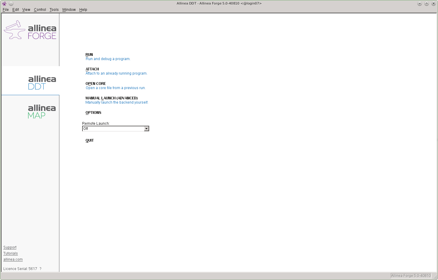
Select Allinea MAP in the tools available box and select Profile.

>

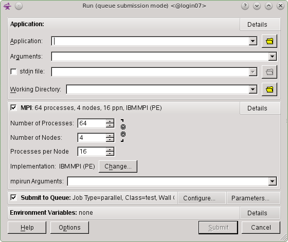
Configure MAP

1. In the Application drop down box select the application you want to profile along with it's directory.

2. In the Arguments box enter the program arguments if any.

3. In the Working Directory drop down box select the directory you want as a working directory, typically the directory where the application is located.

4. Set the MPI configuration.

   1. Set the Number of Processes drop down box.

   2. Set the Number of Nodes drop down box.

   3. Set the Processes per Node drop down box.

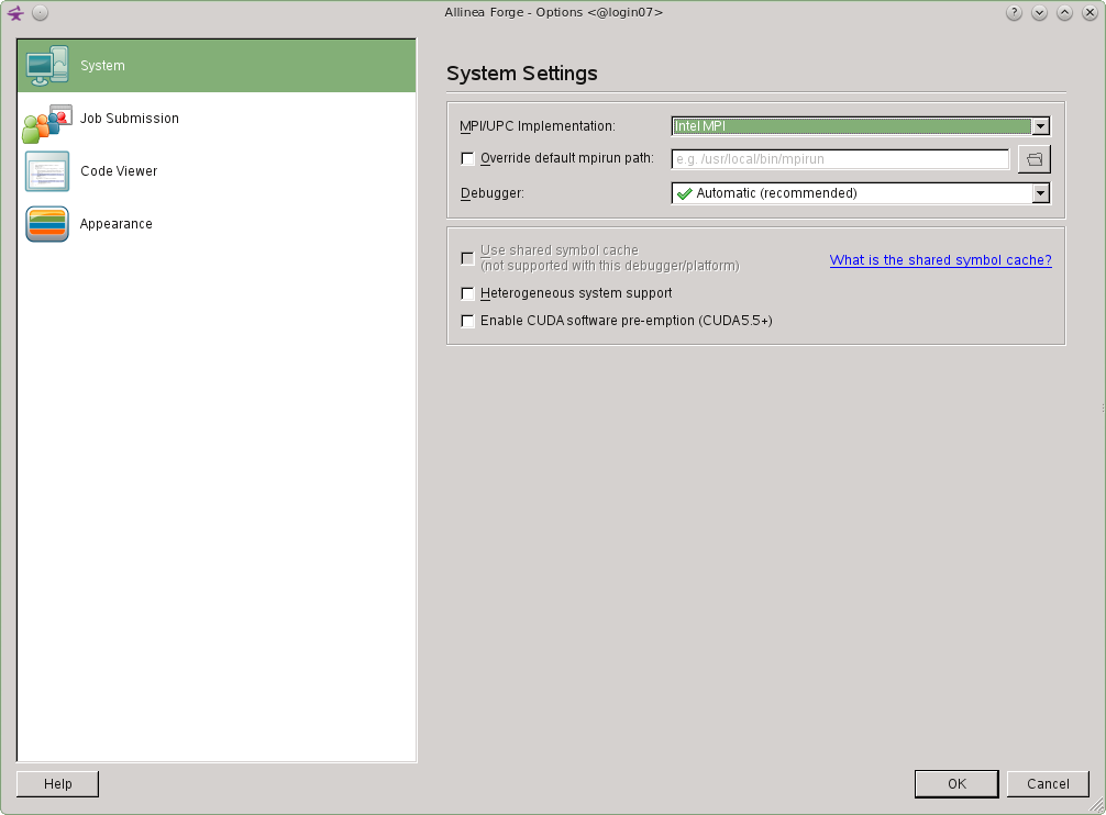
5. Set the MPI implementation you want to use by clicking on the Change button.

   

6. Ensure that the Submit to Queue tick box is selected.

7. Open the Submit to Queue configuration by selecting the Configure tab.

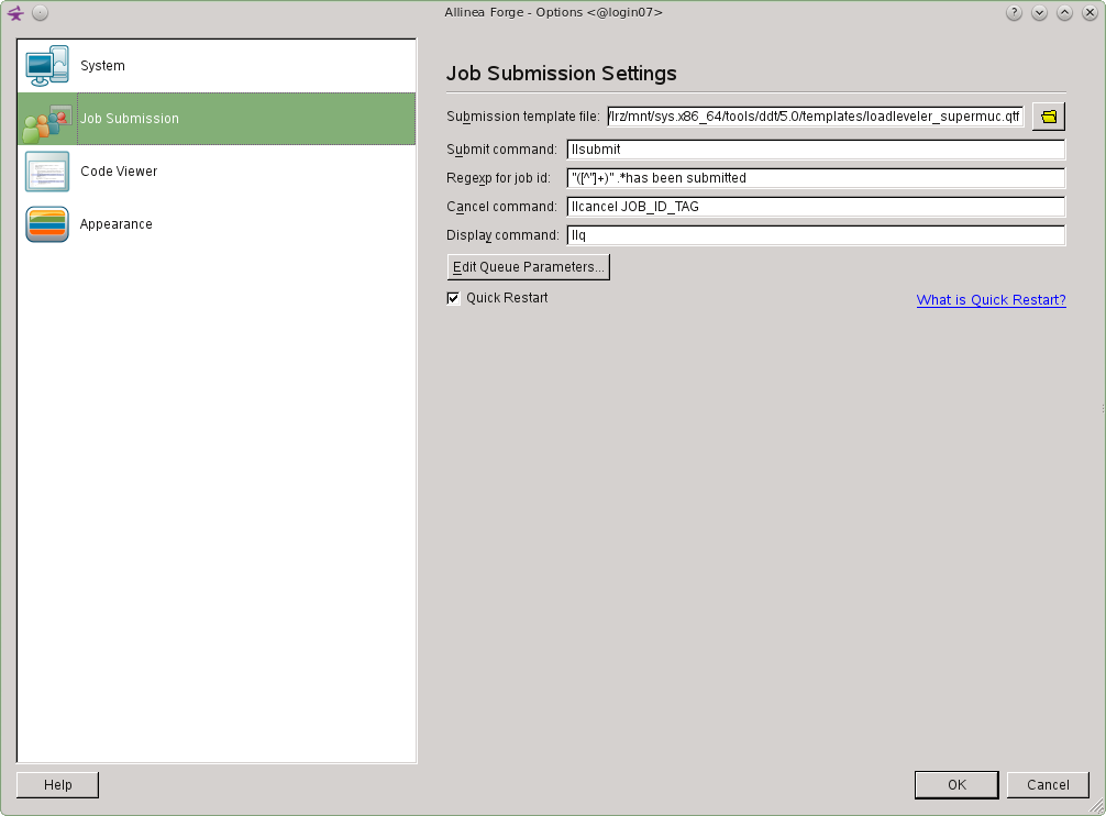
1. In The Submission template file: box ensure that the template file /lrz/mnt/sys.x86_64/tools/ddt/5.0/templates/loadleveler_supermuc.qtf is selected. It is very important that this configuration file is used on SuperMUC. Then select the OK button.

1. Open the Submit to Queue parameters by selecting the Parameter tab.

   

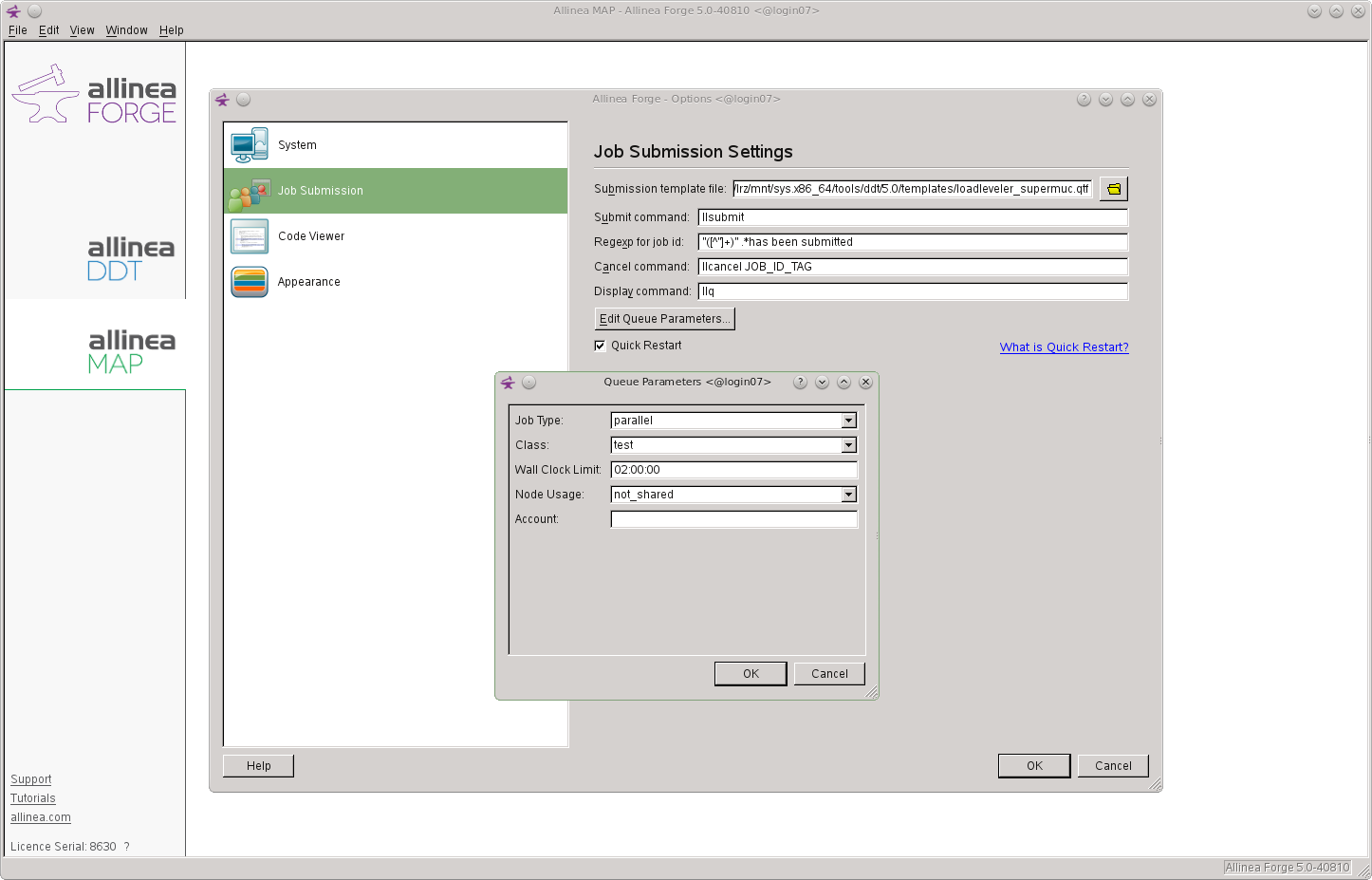
   1. In the Job Type drop down box select MPICH for Intel MPI and parallel for IMB MPI.

   2. In the Class drop down box select which queue on SuperMUC you want the job to be submitted too.

   3. In the Wall Clock Limit box set the time you want the job to run for.

   4. In the Account box set it to the SuperMUC username (account) you want the job to run under. Then press the OK button.

Profiling Results

Once the instrumented applications has been successfully executed, MAP displays the collected data within a GUI.

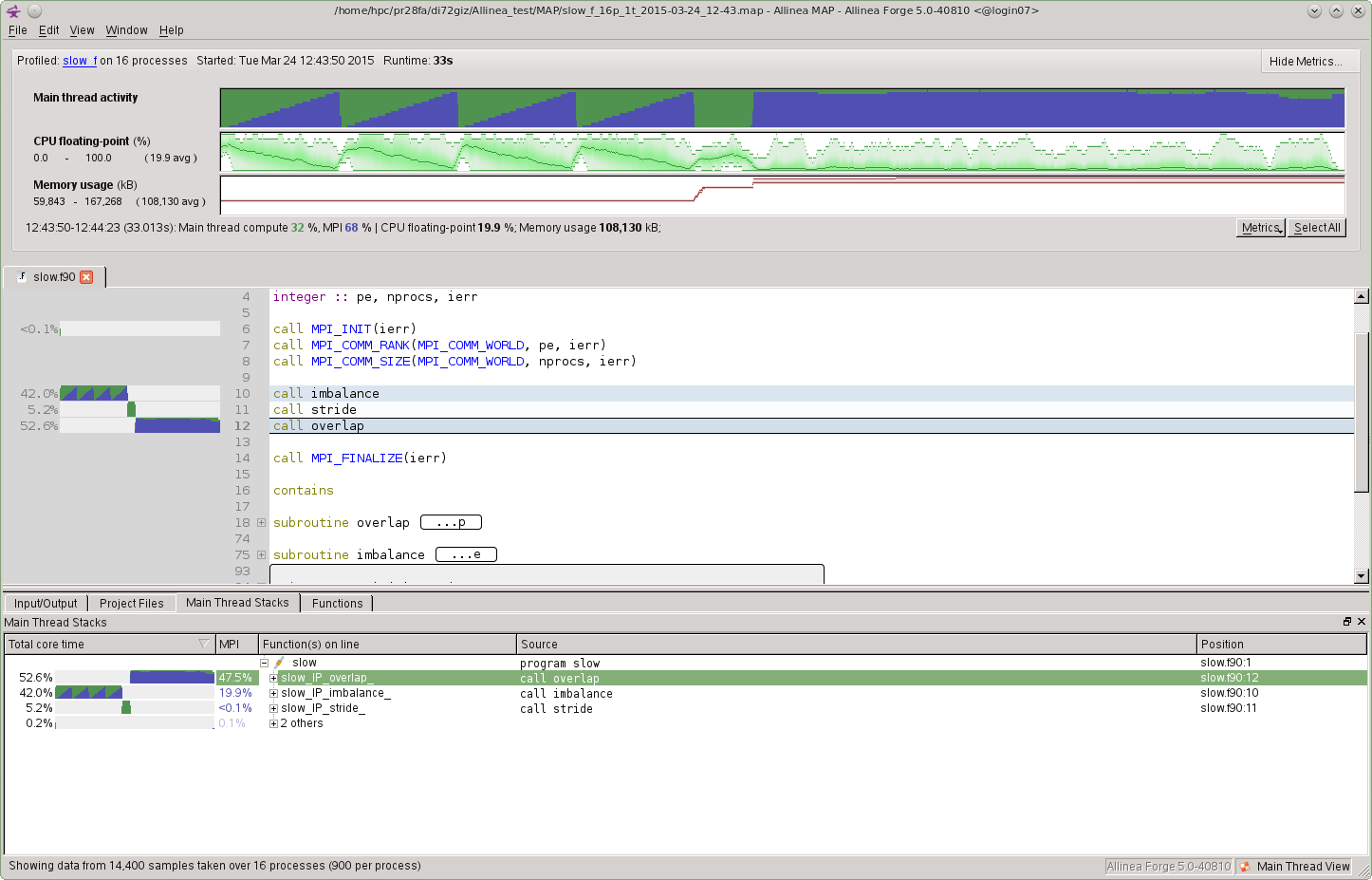
Metric View

The top section shows the "Metrics view," displaying a timeline of a few selected performance data. By default it shows Memory usage (M) for each task's memorage usage, MPI call duration (ms) for the time spent in MPI calls, and CPU floating-point (%) for the percentage of time each rank spends in floating-point CPU instruction.

Each vertical slice shows the distribution of values across (MPI) tasks at the moment. The minimum, maximum and the mean are displayed, and shading gives you an idea about how data is clustered. A region of large load imbalance can be visually identified with a fat shaded region.

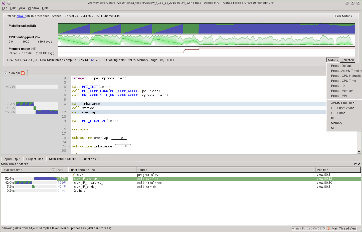
You can add more metrics to the view area by clicking the Metrics button at the bottom and then adding the ones from the list that interest you. Some available ones are Memory usage, MPI call duration, MPI sent, MPI received, MPI calls, MPI point-to-point, MPI collectives, CPU time, CPU memory access, CPU floating-point, CPU floating point vector.

Source Code View

The central displays the source code, which is annotated with performance information to the left of each line. It shows how much total time was spent computing in green and communicating in blue and only lines that spent at least 0.1% of the total time get displayed.

Main thread Stacks

The Main Thread Stacks View is displayed by selecting the Main Thread Stacks tab in the bottom window. This displays a lists the lines where a large wall time was spent, which is sorted by the wall clock time. Clicking on a line results in the code selected view being displayed in the source code window.

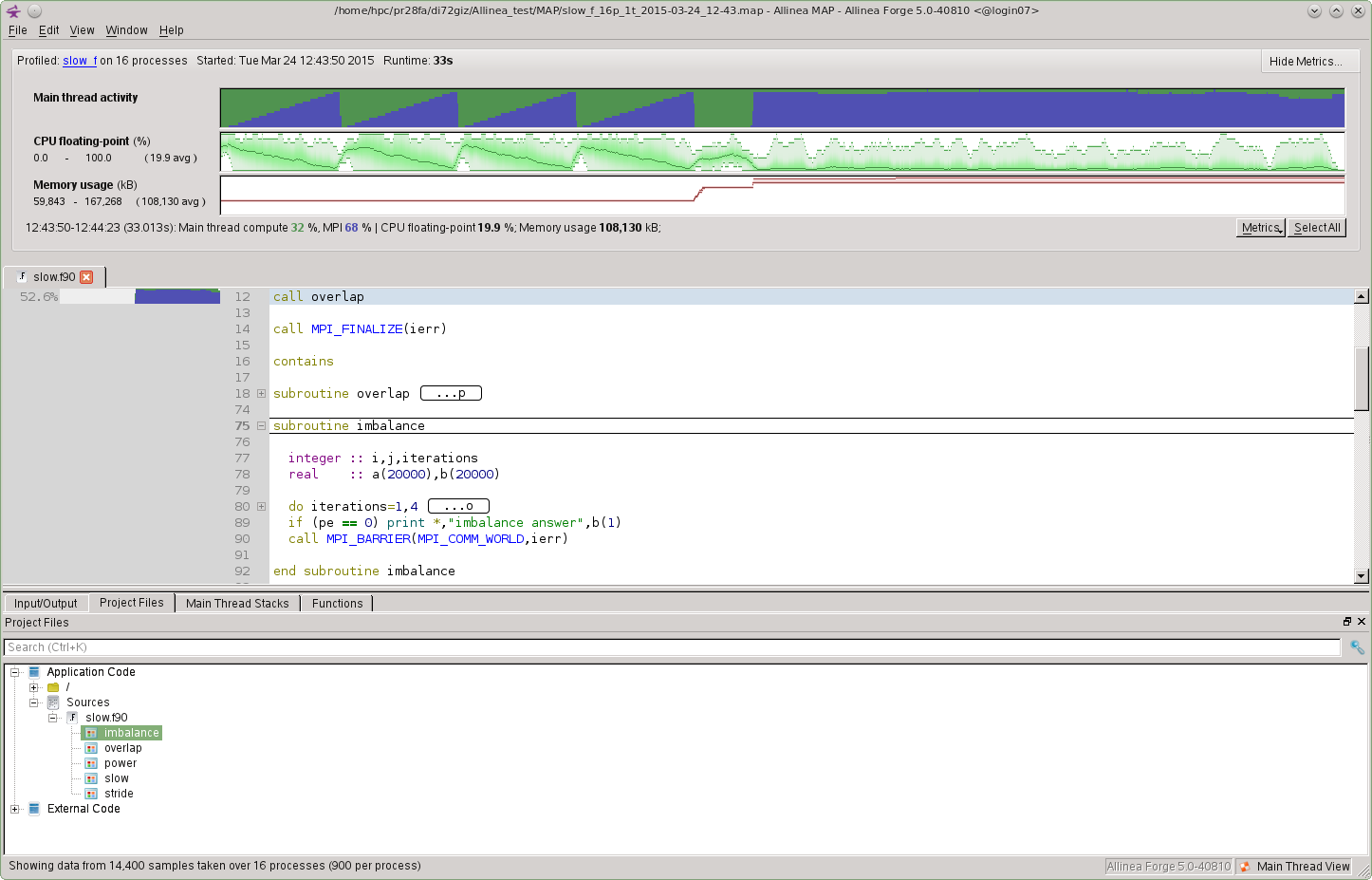
Project Files View

The "Project Files View" area (shown when selecting the Project Files tab) offers a bottom-up view of the performance of your program. Each file, function or folder comes with a time chart that summarily shows how much wall clock time was spent executing code inside that file/function/folder, the External Codeis typically system libraries.

When you hover your mouse over the metrics view area, a thin hairline will appear and distribution information for the selected performance metric will be displayed at the bottom of the metrics view area. Similar hairlines will appear in the source code pane and the bottom pane, and they move in sync with the top hairline.

One can also select a region of interest in the horizontal axis (wall clock time) by clicking the left mouse button, dragging the mouse and then releasing the mouse button. The selected region will appear highlighted. The center and bottom pane's contents will be adjusted by the selection.